Phenotype Exploration

workflowr

• Summary
• Checks
• Past versions

Last updated: 2020-09-27

Checks: 7 0

Knit directory: local_adaptation_sequence/

This reproducible R Markdown analysis was created with workflowr (version 1.6.2). The Checks tab describes the reproducibility checks that were applied when the results were created. The Past versions tab lists the development history.

---

R Markdown file: up-to-date

Great! Since the R Markdown file has been committed to the Git repository, you know the exact version of the code that produced these results.

Environment: empty

Great job! The global environment was empty. Objects defined in the global environment can affect the analysis in your R Markdown file in unknown ways. For reproduciblity it’s best to always run the code in an empty environment.

Seed: set.seed(20200709)

The command set.seed(20200709) was run prior to running the code in the R Markdown file. Setting a seed ensures that any results that rely on randomness, e.g. subsampling or permutations, are reproducible.

Session information: recorded

Great job! Recording the operating system, R version, and package versions is critical for reproducibility.

Cache: none

Nice! There were no cached chunks for this analysis, so you can be confident that you successfully produced the results during this run.

File paths: relative

Great job! Using relative paths to the files within your workflowr project makes it easier to run your code on other machines.

Repository version: c8db4d0

Great! You are using Git for version control. Tracking code development and connecting the code version to the results is critical for reproducibility.

The results in this page were generated with repository version c8db4d0. See the Past versions tab to see a history of the changes made to the R Markdown and HTML files.

Note that you need to be careful to ensure that all relevant files for the analysis have been committed to Git prior to generating the results (you can use wflow_publish or wflow_git_commit). workflowr only checks the R Markdown file, but you know if there are other scripts or data files that it depends on. Below is the status of the Git repository when the results were generated:

Ignored files:
    Ignored:    .Rhistory
    Ignored:    .Rproj.user/
    Ignored:    data/200907_SIM/
    Ignored:    data/200910_RAN/
    Ignored:    data/Bos_taurus.ARS-UCD1.2.101.gtf.gz
    Ignored:    data/Bos_taurus.ARS-UCD1.2.QTL.gff.gz
    Ignored:    data/Johnston_ATAC-seq/
    Ignored:    data/animal_table.rds
    Ignored:    data/prism_climate_data/
    Ignored:    data/prism_dataframe.csv
    Ignored:    data/uszips.csv
    Ignored:    desktop.ini
    Ignored:    output/200822_Lab_IDs.csv
    Ignored:    output/200907_Lab_IDs.csv
    Ignored:    output/200907_SIM/
    Ignored:    output/200909_RAN_Lab_IDs.csv
    Ignored:    output/200910_RAN/200910_RAN.phenotypes.csv
    Ignored:    output/200910_RAN/200910_RAN.phenotypes.txt
    Ignored:    output/200910_RAN/gpsm/
    Ignored:    output/200910_RAN/gwas/
    Ignored:    output/200910_RAN/phenotypes/200910_RAN.info.csv
    Ignored:    output/200910_RAN/phenotypes/200910_RAN.noLSF.allenv.txt
    Ignored:    output/200910_RAN_Lab_IDs.csv
    Ignored:    output/desktop.ini
    Ignored:    output/k10.allvars.seed2.rds
    Ignored:    output/k9.allvars.seed1.rds
    Ignored:    output/k9.allvars.seed2.rds
    Ignored:    output/k9.threevars.seed1.rds
    Ignored:    output/k9.threevars.seed2.rds
    Ignored:    output/kmeans_plotlist.RDS
    Ignored:    output/zipcode_zones.csv

Untracked files:
    Untracked:  analysis/200910_RAN.envGWAS_results.Rmd
    Untracked:  analysis/GPSM.Rmd
    Untracked:  code/countgens_RAN.R
    Untracked:  ftpconfigs/
    Untracked:  functions.R

Unstaged changes:
    Modified:   .ftpconfig
    Modified:   .gitignore
    Modified:   analysis/animal_locations.Rmd
    Modified:   analysis/sex_GWAS.Rmd
    Modified:   code/annotation_functions.R
    Modified:   code/config/200907_SIM.GPSM.config.yaml
    Modified:   code/config/200907_SIM.envGWAS.config.yaml
    Modified:   code/config/200910_RAN.config.yaml
    Modified:   code/config/200910_RAN_noLSF.config.yaml
    Deleted:    data/README.md

Note that any generated files, e.g. HTML, png, CSS, etc., are not included in this status report because it is ok for generated content to have uncommitted changes.

---

These are the previous versions of the repository in which changes were made to the R Markdown (analysis/phenotype_exploration.Rmd) and HTML (docs/phenotype_exploration.html) files. If you’ve configured a remote Git repository (see ?wflow_git_remote), click on the hyperlinks in the table below to view the files as they were in that past version.

File	Version	Author	Date	Message
Rmd	c8db4d0	Troy Rowan	2020-09-27	Fixed issues with the gitignore to make images render
html	d77d694	Troy Rowan	2020-09-27	Build site.
Rmd	c9053dd	Troy Rowan	2020-09-27	Trying to get images to display
html	194bd22	Troy Rowan	2020-09-25	Build site.
Rmd	752c0c1	Troy Rowan	2020-09-25	Trying to get figures to render online
html	1156bd1	Troy Rowan	2020-09-25	Build site.
Rmd	ecef16d	Troy Rowan	2020-09-25	wflow_publish(files = c(“analysis/phenotype_exploration.Rmd”))
Rmd	7dce809	Troy Rowan	2020-09-20	Added file for exploring phenotype distributions

---

Simmental

simmental =
  read_csv("output/200907_SIM/phenotypes/200907_SIM.info.csv") %>%
      mutate(sqrt_age = age^0.5,
             cbrt_age = age^0.333,
             log_age = log(age),
             bc_age = bcPower(age, lambda = 0.0345))

Age Summary Stats

simmental %>% 
  select(age) %>% 
  summarize(mean_age = mean(age, na.rm = TRUE),
            median_age = median(age, na.rm = TRUE),
            sd_age = sd(age, na.rm = TRUE),
            min_age = min(age, na.rm = TRUE),
            max_age = max(age, na.rm = TRUE))

# A tibble: 1 x 5
  mean_age median_age sd_age min_age max_age
     <dbl>      <dbl>  <dbl>   <dbl>   <dbl>
1     5.90       5.06   3.75    1.01    52.5

Transformations to Age:

Untransformed

simmental %>% 
  select(age) %>%
  ggplot()+
  geom_histogram(aes(x = age), mutate(simmental, z = FALSE), bins = 100, fill = "dodgerblue")+
  geom_histogram(aes(x = age), mutate(simmental, z = TRUE), bins = 250, fill = "dodgerblue")+
  theme_cowplot()+
  labs(title = "Simmental Ages\n(Untransformed)", x = "Age (as of 9-15-2020)", y = "Count")+
  facet_zoom(xlim = c(10,45), ylim = c(0,175), zoom.data = z, horizontal = FALSE)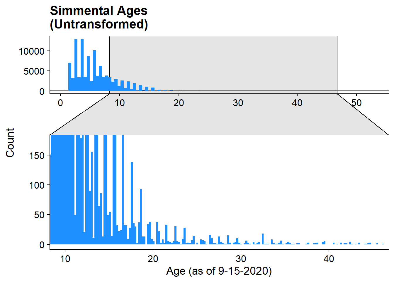

Square Root

simmental%>% 
  ggplot()+
  geom_histogram(aes(x = sqrt_age), mutate(simmental, z = FALSE), bins = 100, fill = "dodgerblue")+
  geom_histogram(aes(x = sqrt_age), mutate(simmental, z = TRUE), bins = 250, fill = "dodgerblue")+
  theme_cowplot()+
  labs(title = "Simmental Ages\n(Square Root Transformed)", x = "Age (as of 9-15-2020)", y = "Count")+
  facet_zoom(xlim = c(3,7), ylim = c(0,175), zoom.data = z, horizontal = FALSE)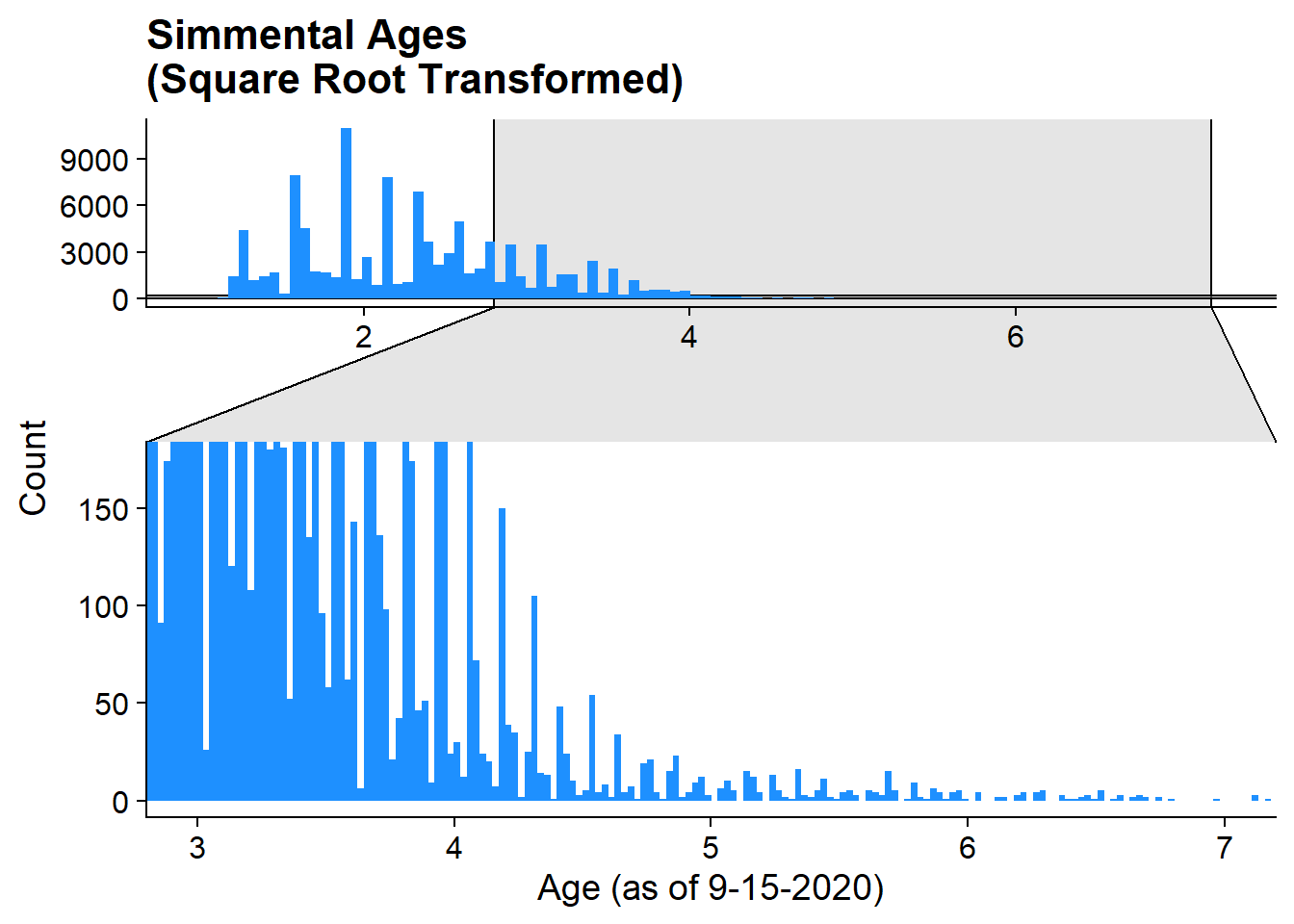

Cube Root

simmental%>% 
  ggplot()+
  geom_histogram(aes(x = cbrt_age), mutate(simmental, z = FALSE), bins = 100, fill = "dodgerblue")+
  geom_histogram(aes(x = cbrt_age), mutate(simmental, z = TRUE), bins = 250, fill = "dodgerblue")+
  theme_cowplot()+
  labs(title = "Simmental Ages\n(Cube Root Transformed)", x = "Age (as of 9-15-2020)", y = "Count")+
  facet_zoom(xlim = c(2,3.6), ylim = c(0,175), zoom.data = z, horizontal = FALSE)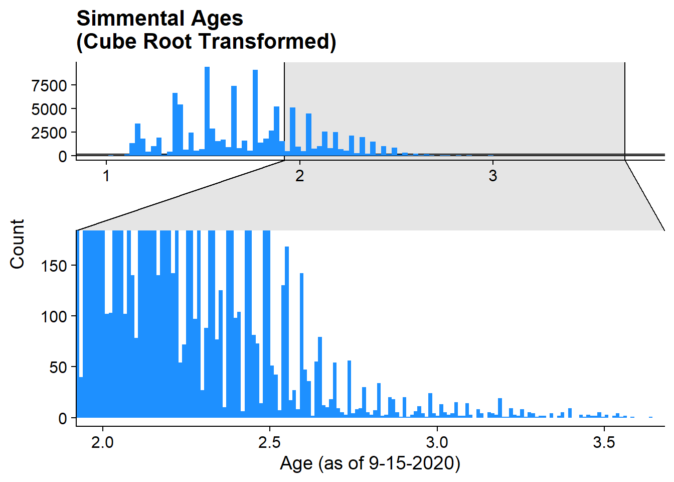

Log

simmental%>% 
  ggplot()+
  geom_histogram(aes(x = log_age), mutate(simmental, z = FALSE), bins = 100, fill = "dodgerblue")+
  geom_histogram(aes(x = log_age), mutate(simmental, z = TRUE), bins = 250, fill = "dodgerblue")+
  theme_cowplot()+
  labs(title = "Simmental Ages\n(log Transformed)", x = "Age (as of 9-15-2020)", y = "Count")+
  facet_zoom(xlim = c(2,3.6), ylim = c(0,175), zoom.data = z, horizontal = FALSE)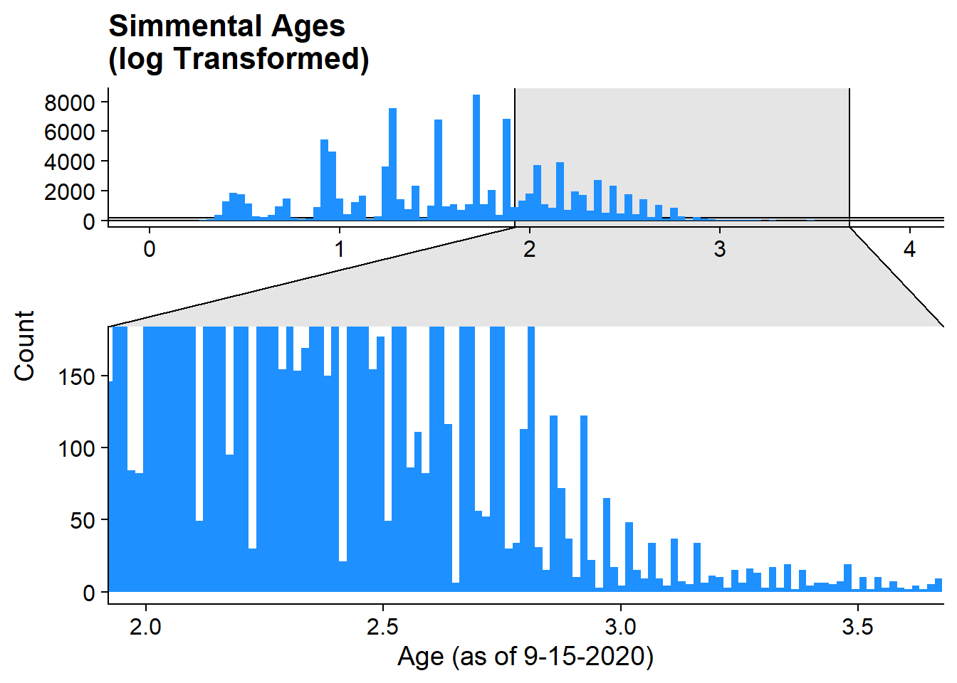

Box-Cox

simmental%>% 
  ggplot()+
  geom_histogram(aes(x = bc_age), mutate(simmental, z = FALSE), bins = 100, fill = "dodgerblue")+
  geom_histogram(aes(x = bc_age), mutate(simmental, z = TRUE), bins = 250, fill = "dodgerblue")+
  theme_cowplot()+
  labs(title = "Simmental Ages\n(Box-Cox Transformed)", x = "Age (as of 9-15-2020)", y = "Count")+
  facet_zoom(xlim = c(2,3.6), ylim = c(0,175), zoom.data = z, horizontal = FALSE)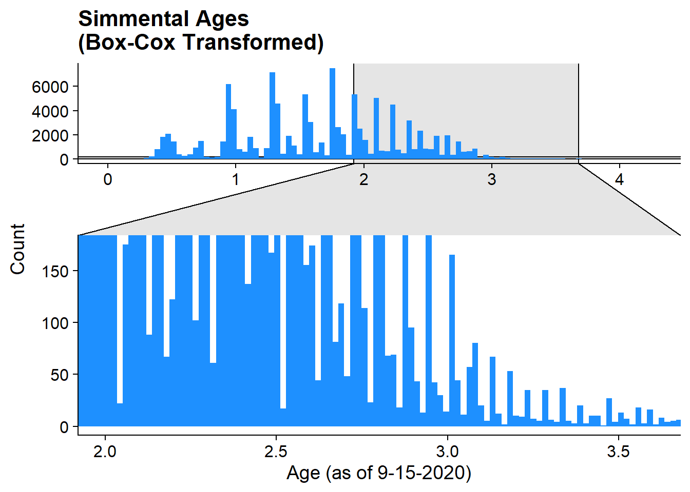

Generation Counts

Summary Stats for Generation Number

Unable to actually calculate this at this point as we haven’t received the updated pedigree from Red Angus

simmental %>%
  select(equiGen, fullGen, maxGen) %>%
  summarize_all(list(mean, median, sd, min, max))%>% 
  gather(key = "key", value = "value") %>%
  separate(key, c("variable", "stat"), sep = "_") %>%
  spread(stat, value) %>% 
  rename(generation_count = variable, mean = fn1, median = fn2, sd = fn3, min = fn4, max = fn5)

# A tibble: 3 x 6
  generation_count  mean median    sd   min   max
  <chr>            <dbl>  <dbl> <dbl> <dbl> <dbl>
1 equiGen           7.26   8.04  2.47     0  11.4
2 fullGen           3.73   4     1.89     0   7  
3 maxGen           16.4   18     4.75     0  23  

Distributions of Generation

equiGen

Note the high number of “zero” generations here. Wondering if we shouldn’t count those as NA if we choose to go this route?

simmental%>% 
  ggplot()+
  geom_histogram(aes(x = equiGen), bins = 100, fill = "dodgerblue")+
  theme_cowplot()+
  labs(title = "Simmental Equivalent Generations", x = "Age (as of 9-15-2020)", y = "Count")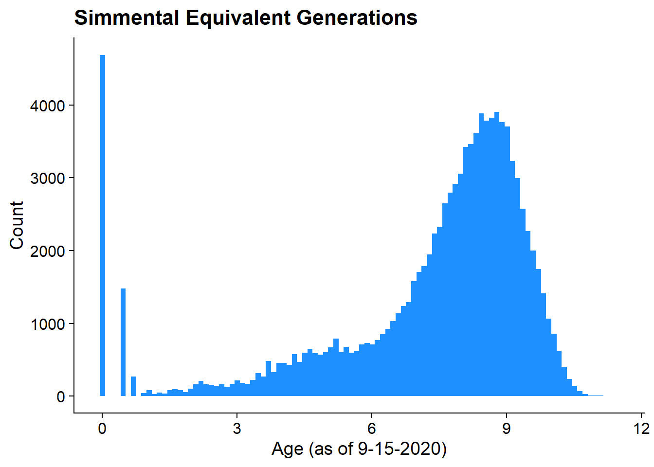

equiGen squared

simmental%>% 
  ggplot()+
  geom_histogram(aes(x = equiGen^2), bins = 100, fill = "dodgerblue")+
  theme_cowplot()+
  labs(title = "Simmental Equivalent Generations Squared", x = "Age (as of 9-15-2020)", y = "Count")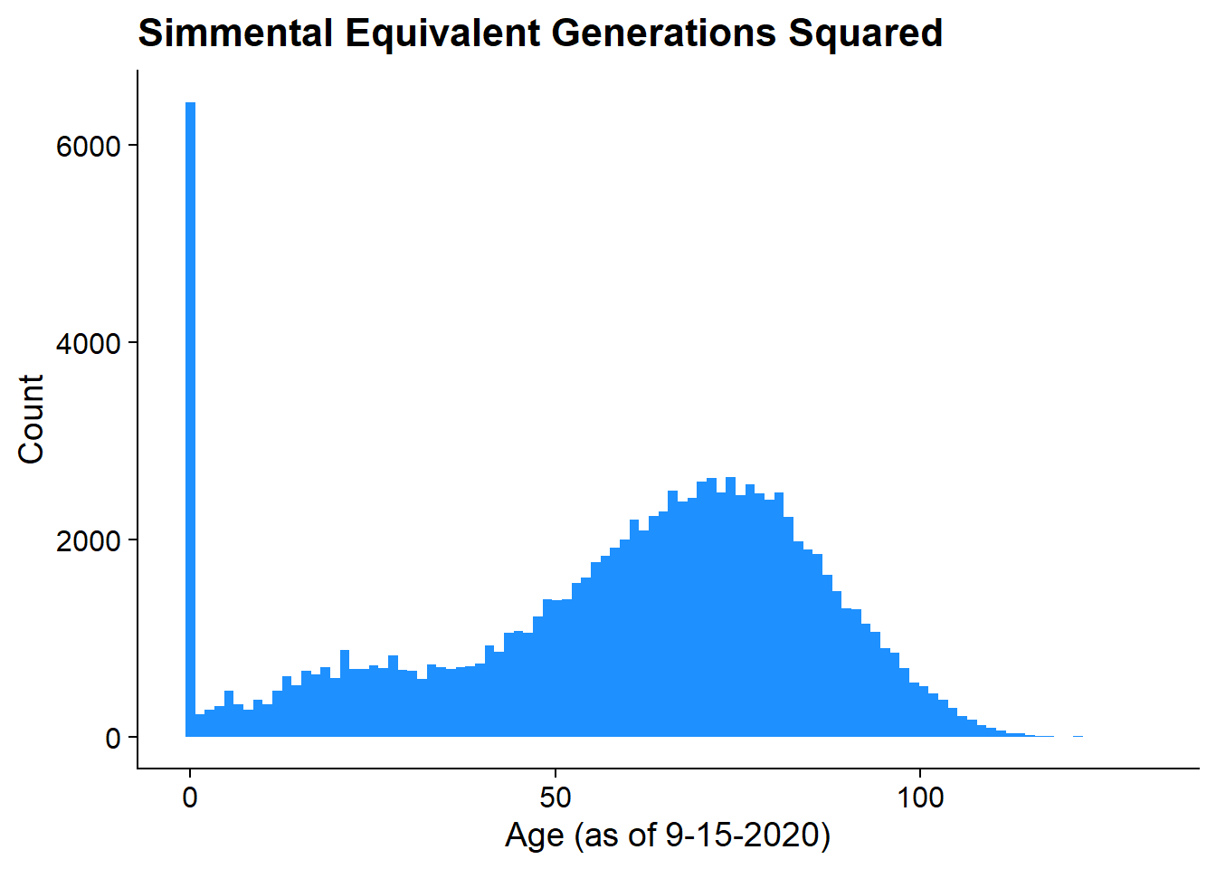

fullGen

simmental%>% 
  ggplot()+
  geom_histogram(aes(x = fullGen),  bins = 10, fill = "dodgerblue")+
  theme_cowplot()+
  labs(title = "Simmental Full Generations", x = "Age (as of 9-15-2020)", y = "Count")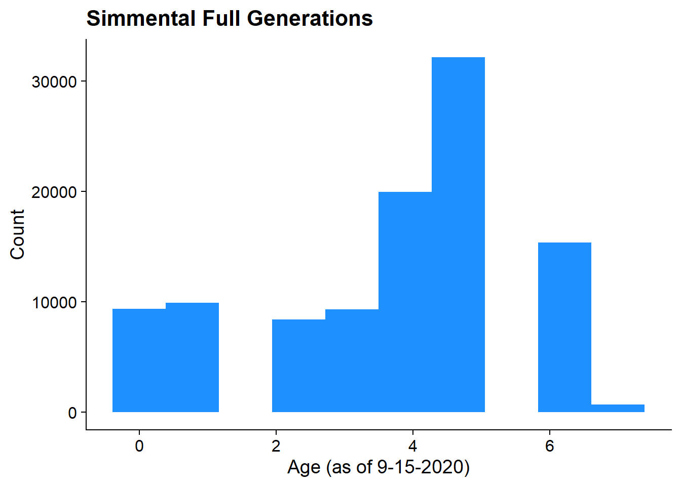

maxGen

simmental%>% 
  ggplot()+
  geom_histogram(aes(x = maxGen),  bins = 25, fill = "dodgerblue")+
  theme_cowplot()+
  labs(title = "Simmental Max Generations", x = "Age (as of 9-15-2020)", y = "Count")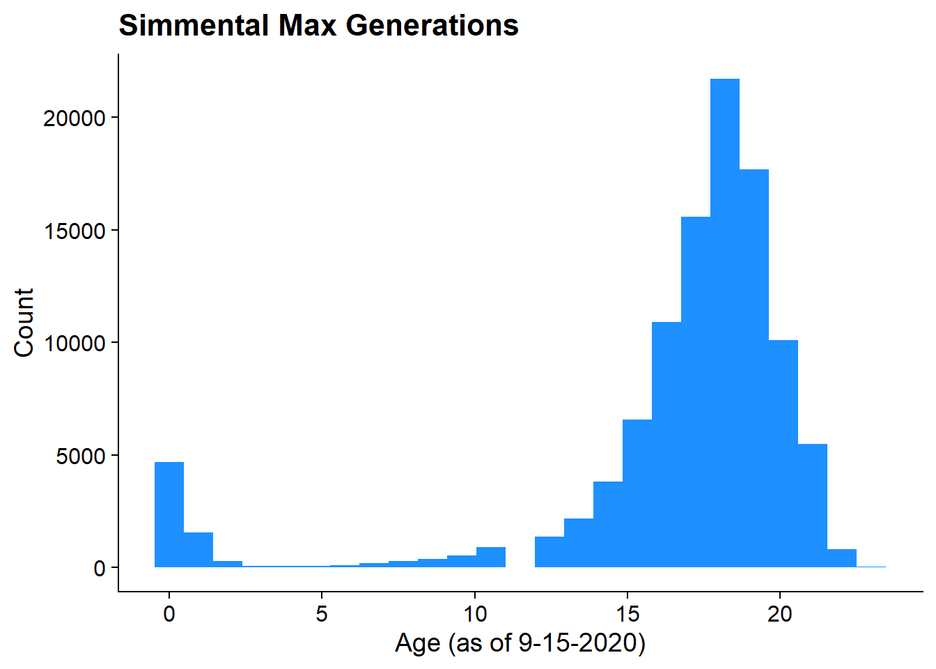

Red Angus

redangus = read_csv("output/200910_RAN/phenotypes/200910_RAN.info.csv")

Exploring Generation Proxy Phenotypes

Calculating Generation Number

countGen(
  data.frame(
    id = 1:5,
    dam = c(0,0,1,1,4),
    sire = c(0,0,2,2,3)
  )
)

ran_ped = 
  read_csv("data/200910_RAN/All_Animals_SireDam.csv") %>% 
  select(id = anm_key, sire = sire_key, dam = dam_key) %>% 
  replace_na(list(sire = 0, dam = 0))

ran_ped = 
  orderPed(ran_ped)

Age Summary Stats

redangus %>% 
  select(age) %>% 
  summarize(mean_age = mean(age, na.rm = TRUE),
            median_age = median(age, na.rm = TRUE),
            sd_age = sd(age, na.rm = TRUE),
            min_age = min(age, na.rm = TRUE),
            max_age = max(age, na.rm = TRUE))

# A tibble: 1 x 5
  mean_age median_age sd_age min_age max_age
     <dbl>      <dbl>  <dbl>   <dbl>   <dbl>
1     4.37       3.59   3.07   0.902    45.5

Transformations to Age:

Untransformed

ages = 
  redangus %>% 
    select(age) %>%
    mutate(sqrt_age = age^0.5,
           cbrt_age = age^0.333,
           log_age = log(age),
           bc_age = bcPower(age, lambda = -0,237)
           )


  
redangus %>% 
  select(age) %>%
  ggplot()+
  geom_histogram(aes(x = age), mutate(redangus, z = FALSE), bins = 100, fill = "indianred")+
  geom_histogram(aes(x = age), mutate(redangus, z = TRUE), bins = 250, fill = "indianred")+
  theme_cowplot()+
  labs(title = "Red Angus Ages\n(Untransformed)", x = "Age (as of 9-15-2020)", y = "Count")+
  facet_zoom(xlim = c(10,45), ylim = c(0,175), zoom.data = z, horizontal = FALSE)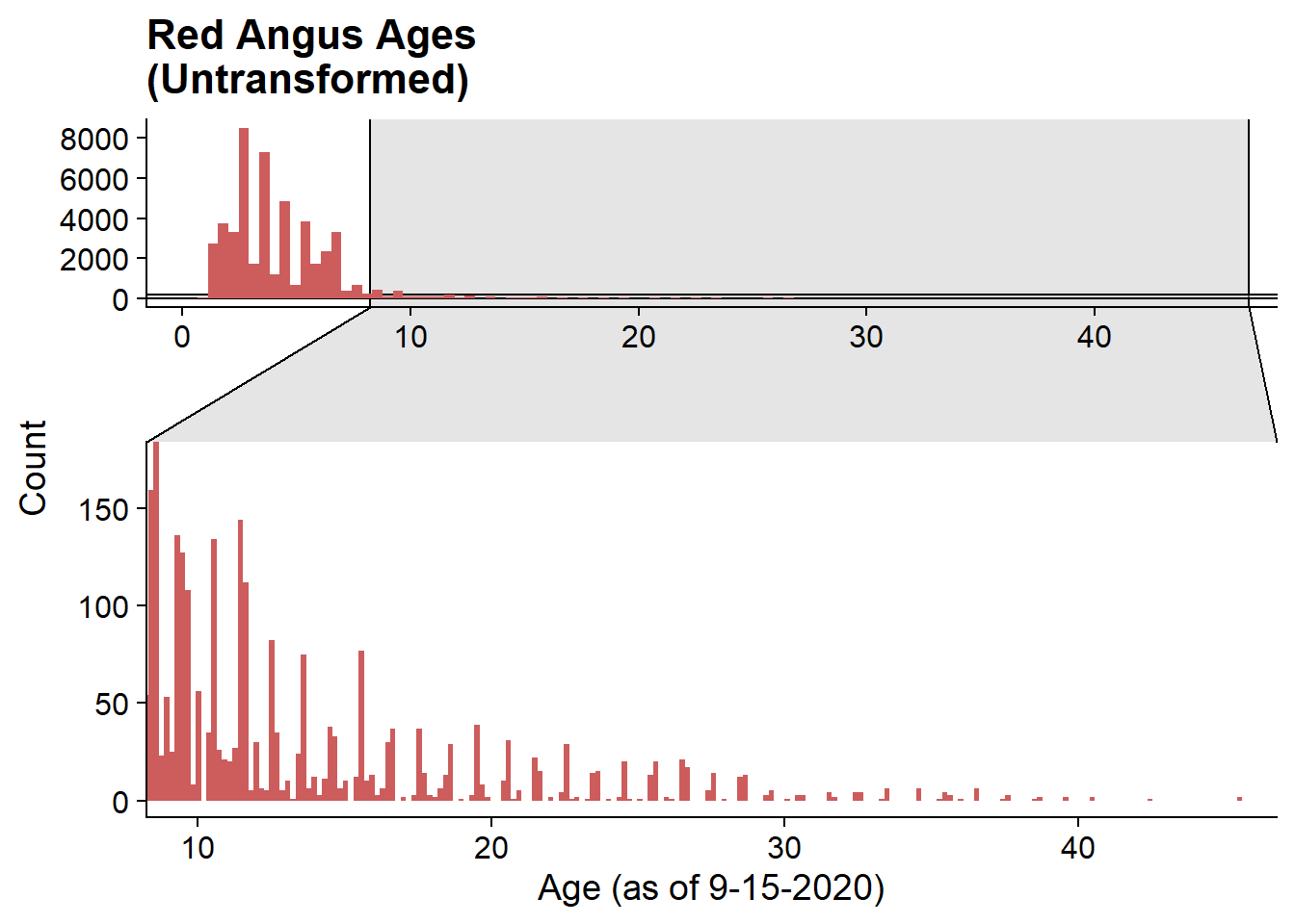

Square Root

ages%>% 
  ggplot()+
  geom_histogram(aes(x = sqrt_age), mutate(ages, z = FALSE), bins = 100, fill = "indianred")+
  geom_histogram(aes(x = sqrt_age), mutate(ages, z = TRUE), bins = 250, fill = "indianred")+
  theme_cowplot()+
  labs(title = "Red Angus Ages\n(Square Root Transformed)", x = "Age (as of 9-15-2020)", y = "Count")+
  facet_zoom(xlim = c(3,7), ylim = c(0,175), zoom.data = z, horizontal = FALSE)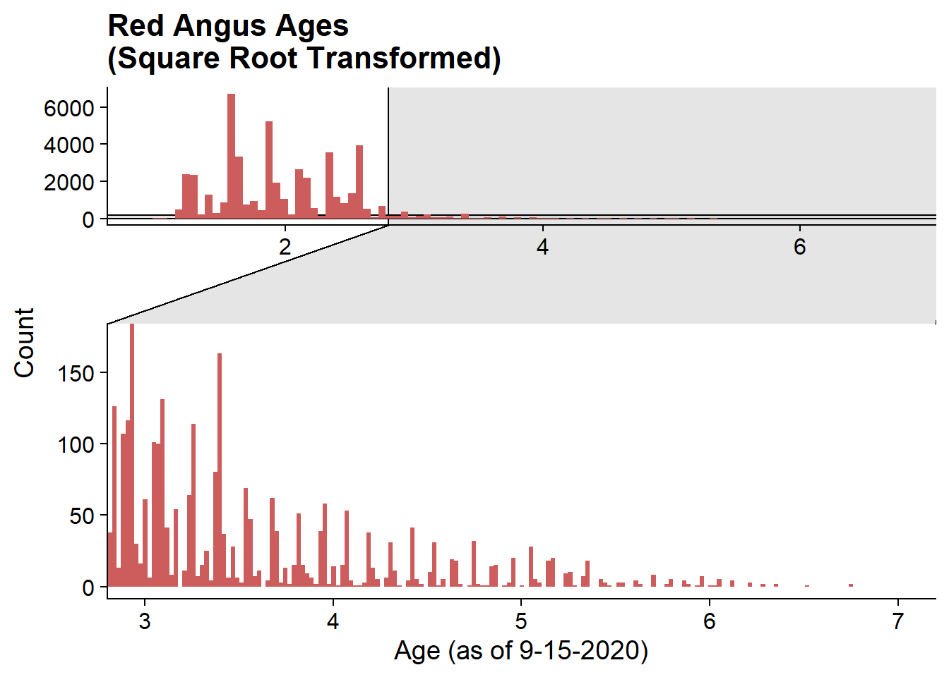

Cube Root

ages%>% 
  ggplot()+
  geom_histogram(aes(x = cbrt_age), mutate(ages, z = FALSE), bins = 100, fill = "indianred")+
  geom_histogram(aes(x = cbrt_age), mutate(ages, z = TRUE), bins = 250, fill = "indianred")+
  theme_cowplot()+
  labs(title = "Red Angus Ages\n(Cube Root Transformed)", x = "Age (as of 9-15-2020)", y = "Count")+
  facet_zoom(xlim = c(2,3.6), ylim = c(0,175), zoom.data = z, horizontal = FALSE)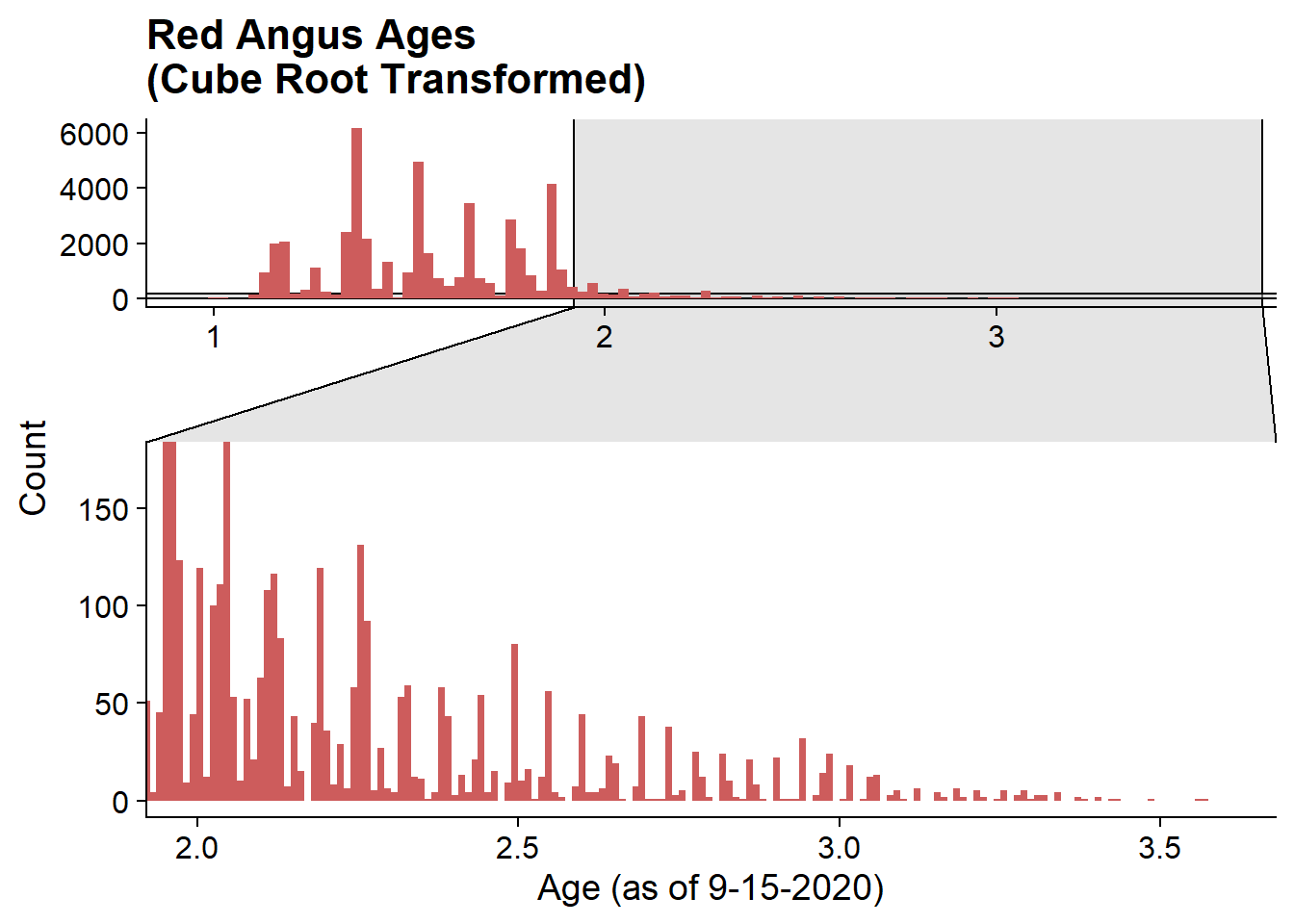

Log

ages%>% 
  ggplot()+
  geom_histogram(aes(x = log_age), mutate(ages, z = FALSE), bins = 100, fill = "indianred")+
  geom_histogram(aes(x = log_age), mutate(ages, z = TRUE), bins = 250, fill = "indianred")+
  theme_cowplot()+
  labs(title = "Red Angus Ages\n(log Transformed)", x = "Age (as of 9-15-2020)", y = "Count")+
  facet_zoom(xlim = c(2,3.6), ylim = c(0,175), zoom.data = z, horizontal = FALSE)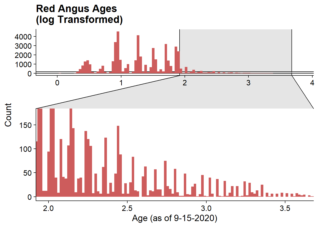

Box-Cox

ages%>% 
  ggplot()+
  geom_histogram(aes(x = bc_age), mutate(ages, z = FALSE), bins = 100, fill = "indianred")+
  geom_histogram(aes(x = bc_age), mutate(ages, z = TRUE), bins = 250, fill = "indianred")+
  theme_cowplot()+
  labs(title = "Red Angus Ages\n(Box-Cox Transformed)", x = "Age (as of 9-15-2020)", y = "Count")+
  facet_zoom(xlim = c(2,3.6), ylim = c(0,175), zoom.data = z, horizontal = FALSE)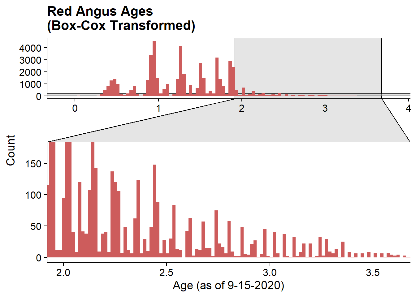

Summary Stats for Generation Number

Unable to actually calculate this at this point as we haven’t received the updated pedigree from Red Angus

# redangus %>% 
#   select(age) %>% 
#   summarize(mean_age = mean(age, na.rm = TRUE),
#             median_age = median(age, na.rm = TRUE),
#             sd_age = sd(age, na.rm = TRUE),
#             min_age = min(age, na.rm = TRUE),
#             max_age = max(age, na.rm = TRUE))

Session information

sessionInfo()

R version 4.0.2 (2020-06-22)
Platform: x86_64-w64-mingw32/x64 (64-bit)
Running under: Windows 10 x64 (build 19041)

Matrix products: default

locale:
[1] LC_COLLATE=English_United States.1252 
[2] LC_CTYPE=English_United States.1252   
[3] LC_MONETARY=English_United States.1252
[4] LC_NUMERIC=C                          
[5] LC_TIME=English_United States.1252    

attached base packages:
[1] stats     graphics  grDevices utils     datasets  methods   base     

other attached packages:
 [1] car_3.0-9        carData_3.0-4    optiSel_2.0.3    EnvStats_2.3.1  
 [5] forcats_0.5.0    stringr_1.4.0    dplyr_1.0.2      readr_1.3.1     
 [9] tidyr_1.1.2      tibble_3.0.3     tidyverse_1.3.0  ggforce_0.3.2   
[13] pedigree_1.4     reshape_0.8.8    HaploSim_1.8.4   Matrix_1.2-18   
[17] lubridate_1.7.9  here_0.1         factoextra_1.0.7 ggplot2_3.3.2   
[21] purrr_0.3.4      cowplot_1.1.0    ggthemes_4.2.0   maps_3.3.0      
[25] knitr_1.30       workflowr_1.6.2 

loaded via a namespace (and not attached):
  [1] colorspace_1.4-1        rio_0.5.16              ellipsis_0.3.1         
  [4] rprojroot_1.3-2         fs_1.5.0                rstudioapi_0.11        
  [7] farver_2.0.3            ggrepel_0.8.2           fansi_0.4.1            
 [10] xml2_1.3.2              codetools_0.2-16        doParallel_1.0.15      
 [13] shapes_1.2.5            polyclip_1.10-0         optiSolve_0.1.2        
 [16] jsonlite_1.7.1          nloptr_1.2.2.2          kinship2_1.8.5         
 [19] broom_0.7.0             dbplyr_1.4.4            shiny_1.5.0            
 [22] compiler_4.0.2          httr_1.4.2              backports_1.1.10       
 [25] assertthat_0.2.1        fastmap_1.0.1           cli_2.0.2              
 [28] later_1.1.0.1           tweenr_1.0.1            htmltools_0.5.0        
 [31] tools_4.0.2             gtable_0.3.0            glue_1.4.2             
 [34] reshape2_1.4.4          Rcpp_1.0.5              cellranger_1.1.0       
 [37] vctrs_0.3.4             iterators_1.0.12        crosstalk_1.1.0.1      
 [40] xfun_0.17               openxlsx_4.2.2          rvest_0.3.6            
 [43] mime_0.9                miniUI_0.1.1.1          lifecycle_0.2.0        
 [46] ECOSolveR_0.5.3         nadiv_2.16.2.0          MASS_7.3-53            
 [49] scales_1.1.1            hms_0.5.3               promises_1.1.1         
 [52] parallel_4.0.2          curl_4.3                yaml_2.2.1             
 [55] stringi_1.5.3           foreach_1.5.0           zip_2.1.1              
 [58] manipulateWidget_0.10.1 rlang_0.4.7             pkgconfig_2.0.3        
 [61] rgl_0.100.54            evaluate_0.14           lattice_0.20-41        
 [64] labeling_0.3            htmlwidgets_1.5.1       tidyselect_1.1.0       
 [67] plyr_1.8.6              magrittr_1.5            R6_2.4.1               
 [70] generics_0.0.2          DBI_1.1.0               foreign_0.8-80         
 [73] pillar_1.4.6            haven_2.3.1             whisker_0.4            
 [76] withr_2.3.0             scatterplot3d_0.3-41    abind_1.4-5            
 [79] cccp_0.2-4              pspline_1.0-18          modelr_0.1.8           
 [82] crayon_1.3.4            utf8_1.1.4              alabama_2015.3-1       
 [85] rmarkdown_2.3           grid_4.0.2              readxl_1.3.1           
 [88] minpack.lm_1.2-1        data.table_1.13.0       blob_1.2.1             
 [91] git2r_0.27.1            reprex_0.3.0            digest_0.6.25          
 [94] webshot_0.5.2           xtable_1.8-4            httpuv_1.5.4           
 [97] numDeriv_2016.8-1.1     munsell_0.5.0           magic_1.5-9            
[100] quadprog_1.5-8